An Introduction to Sysquake LE

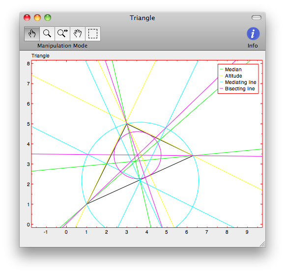
Sysquake is as an awesome program. It is similar to MATLAB, and its language, LME, is mostly compatible with MATLAB code. Overall, it seems Sysquake is mainly geared towards making interactive graphics. As an example, above is an example of the interactive graphics Sysquake can handle. It’s an SQ file that comes with the program. With the mouse, you move one of three points on the plot and it calculated all the radii defined by the triangle.

A Short Tutorial

First, download and install Sysquake LE (the free version).

In this tutorial, we’re going to plot cos(t)  for t equals 0 to 2*pi.

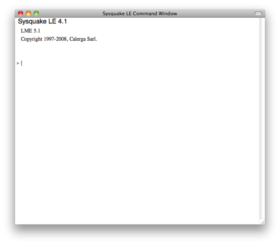
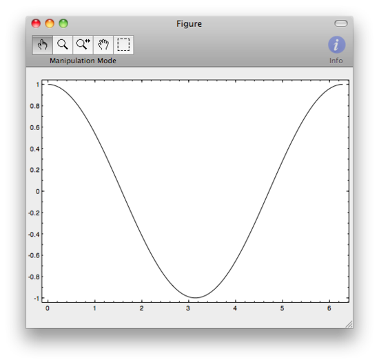
1. When you open Sysquake you are presented with a blank plot window and a command prompt.
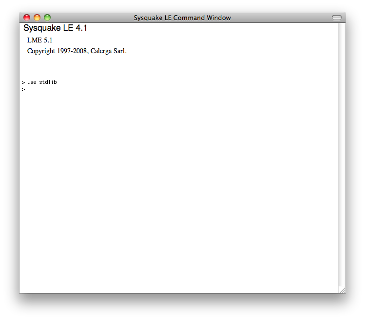
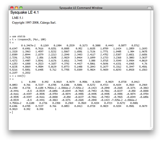
2. Type in use stdlib. Hit enter. This is similar to the ‘include’ statement in some languages, and gives up acces to the our next command.
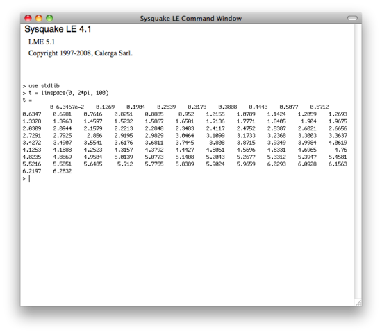
3. Now type in t = linspace(0, 2*pi, 100) followed by enter. This will build a 100 element linearly-spaced 1 dimension matrix of numbers from 0 to 2*pi.



4. Next type x = cos(t) followed by enter. On screen you’re see the results, which is a matrix of exact dimensions as t, but now filled with the cos(t).
   



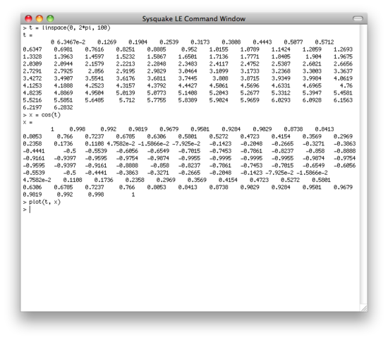
5. We now have two matrices in memory, t and x. I don’t know about you, but I have a hard time visualizing raw numbers, so let’s plot these numbers and see what we get. Type plot(t, x) followed by enter. It may seem weird, but the horizontal axis, in this case t, is entered first, then the vertical. And there we are. We have a plot.





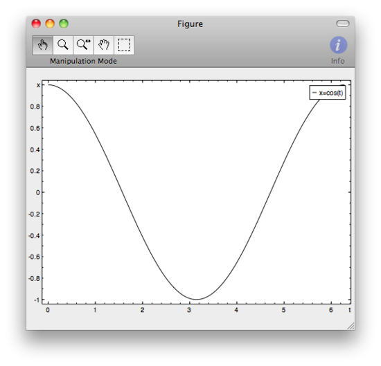
6. We could stop there, but let’s put some finishing touches on out plot. You should really get into the habit of labeling all your plots, axis, legends, titles, etc. It may seem like a pain in the ass, and is quite frankly, but in coming lessons we’ll learn ways to reduce how much we need to type to make great looking plots. Anyways, lets label out axis. Type label(‘t’, ‘x’) and hit enter. You’ll see that we now have labels for our vertical and horizontal axes.
7. Now for out final touch, type legend(‘x=cos(t)’) and hit enter. You’re done, you have a great looking full cycle plot of cosine.