Entries by Jay Kickliter (23)

Friday
Nov122010

11 inch MacBook Air and Autocad

I’m here at an Apple store, and after getting an employee to enter the administrator password, I installed AutoCad for Mac. And in case anyone is wondering, it runs with only 2 GB of RAM. Here’s the proof: 


It did take several beats to start up, but once running, it seemed quite usable. But keep in mind I spent less than 10 minutes with it. In the end, I decided to order the the base 11” Air with the $90 4 GB upgrade, since the RAM is hardwired to the logic-board. It turns out that the SSD storage is removable, and Toshiba will be selling it, so I’m going to keep with 64 GB of storage for now.

Tuesday
Nov092010

Transistor Shunt Voltage Regulator

My buddies Frank, Joe, and I had some time to kill today so we decided to build a transistor shunt voltage regulator. We didn’t know correct terminology of the circuit topology at the time, and therefore couldn’t find any examples on the internet. But, we knew the basic topology of the circuit, and had plenty of transistors and zener diodes laying around, so we came up with the circuit shown in Figure 1. Again, we were shooting in the dark, so had to pick out components on gut feel and trial and error, but for a DC sweep to plot input/output characteristics we settled on Rs = 100 Ω, Rl = 470 Ω, a 13 V zener diode, and a 2N2219 NPN transistor.

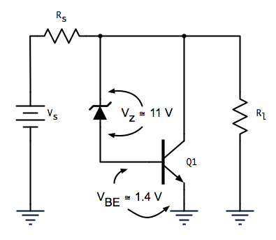
Figure 1—-Transistor Shunt Voltage Regulator

Now, something strange happened when we stepped Vin up from 10—20 V. From Vin = 10—15, Vout increased linearly, just as any voltage divider would. That is, since the zener hadn’t ‘turned on’, the transistor wasn’t sinking any current, and all the current was flowing through Rs and the load. But, when we increased Vin to 16 V, there was a sudden drop in Vout from 12.37 V to 8.50 V. We were puzzled, especially since it appeared as though the circuit was regulating after that, but at a much lower voltage than expected. The end result being plot of Vout/Vin with a strange dip it in (Figure 2). Even weirder, there appeared to be some hysteresis, or memory in the circuit, the plot of the DC sweep from 10—20 V does not match the plot of the sweep from 20—10 V.

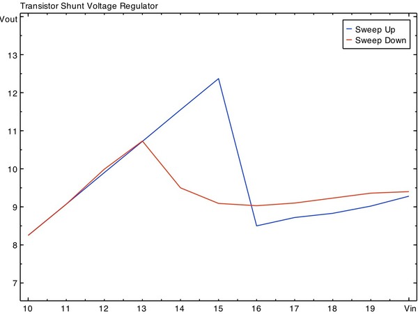
Figure 2—-Original circuit DC sweeps


In comes our professor, Dr. Amani. He suggested adding some series resistance, in this case a 1k Ω chosen randomly (Figure 3). The result? A a very nice regulating curve (Figure 4), which was nearly identical in both 10—20 V and 20—10 V.

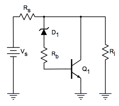
Figure 3—-Rb added to original circuit


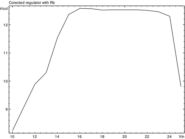
Figure 4—-Correct circuit DC sweep

Why did the circuit need that resistor? And why did the original circuit have memory? I’m still trying to figure it out.

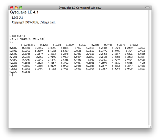
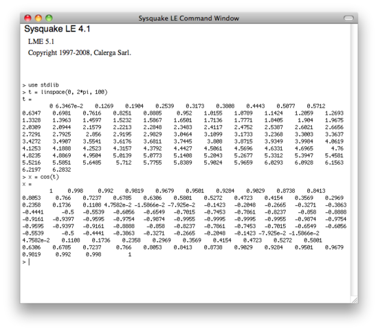
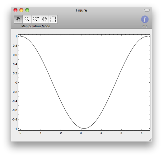
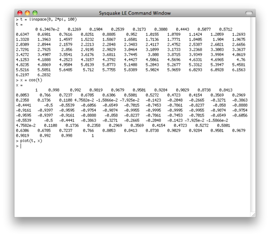
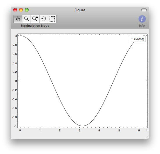
Download the Sysquake files used to create the plots.

Monday
Nov082010

An Introduction to Sysquake LE

Sysquake is as an awesome program. It is similar to MATLAB, and its language, LME, is mostly compatible with MATLAB code. Overall, it seems Sysquake is mainly geared towards making interactive graphics. As an example, above is an example of the interactive graphics Sysquake can handle. It’s an SQ file that comes with the program. With the mouse, you move one of three points on the plot and it calculated all the radii defined by the triangle.

A Short Tutorial

First, download and install Sysquake LE (the free version).

In this tutorial, we’re going to plot cos(t)  for t equals 0 to 2*pi.


  1. When you open Sysquake you are presented with a blank plot window and a command prompt.
  2. Type in use stdlib. Hit enter. This is similar to the ‘include’ statement in some languages, and gives up acces to the our next command.
  3. Now type in t = linspace(0, 2*pi, 100) followed by enter. This will build a 100 element linearly-spaced 1 dimension matrix of numbers from 0 to 2*pi.
  4. Next type x = cos(t) followed by enter. On screen you’re see the results, which is a matrix of exact dimensions as t, but now filled with the cos(t).
  5. We now have two matrices in memory, t and x. I don’t know about you, but I have a hard time visualizing raw numbers, so let’s plot these numbers and see what we get. Type plot(t, x) followed by enter. It may seem weird, but the horizontal axis, in this case t, is entered first, then the vertical. And there we are. We have a plot.
  6. We could stop there, but let’s put some finishing touches on out plot. You should really get into the habit of labeling all your plots, axis, legends, titles, etc. It may seem like a pain in the ass, and is quite frankly, but in coming lessons we’ll learn ways to reduce how much we need to type to make great looking plots. Anyways, lets label out axis. Type label(‘t’, ‘x’) and hit enter. You’ll see that we now have labels for our vertical and horizontal axes.
  7. Now for out final touch, type legend(‘x=cos(t)’) and hit enter. You’re done, you have a great looking full cycle plot of cosine.